
Covariance and Correlation
Statistical quantities for variables relationships


A common problem in statistics is to assess how strongly two random variables and are related to each other. Let and be the respective expected values of X and Y. We assume that expected values mentioned in this article from now on exist (the expected value does not exist for random variables having “large tails” distributions, such as the Cauchy distribution).
Covariance
The covariance between two random variables and is defined as
i.e. for discrete variables
where and vary in the range of their respective variables and ; for continuous variables
Consider the discrete case. One can easily see that given a point , the absolute value of the product represents the area of a rectangle. So we sum positive and negative quantities (taking into account that these are multiplied by a positive weight ) that we can consider — for convenience — as “negative” and “positive” rectangles areas. A linear pattern emerges if there is a clear dominance of positive signed rectangles (depicted below in beige) over negative signed rectangles (depicted below in orange), or – viceversa – when there is a clear dominance of negative signed rectangles over positive ones.

Covariance is large and positive when there is a strong positive relation between the variables: large values of tend to occur with large values of . Covariance is near to zero if datapoints are scattered and no particular trend emerges. Covariance is negative when there is a strong negative relation between variables (higher values of tend to occur with lower values of ). Covariance ranges between and . To be precise, it can be proved that
Correlation
We can normalize in order to constrain covariance between and obtaining the correlation (often cited as Pearson’s correlation coefficient) between variables and
provided that the standard deviations and are nonzero. Here and denote the standard deviations of and . The following picture shows some datasets and their relative correlation coefficients.

Uncorrelation is not independence
When Cov(X, Y) = 0, we say that X and Y are uncorrelated. However, uncorrelation is not independence. Consider two random variables X and Y. The pair (X, Y) takes the values (-1,0), (0,1), (1,0) and (0,-1), each with probability 1/4, as shown in the figure below.
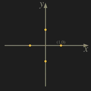
The marginal probability mass functions of X and Y are symmetric around the origin, so their respective expectations E[X] and E[Y] are 0. Furthermore, one coordinate of each of the points is 0, so XY=0 and E[XY] = 0. Therefore
and X, Y are uncorrelated. However, the variables are not independent since a nonzero value of X fixes the value of Y to zero.
Useful links
Nice page on Covariance.
Wikipedia page on Correlation.
Page about the difference between Covariance and Correlation.