


Mixture of Experts from scratch
Conditional computation at your fingertips


This is a simple implementation of the Mixture of Experts (MoE) technique applied to language modeling tasks.
Evaluation and training of deep models can be computationally expensive and time-consuming. The Conditional Computation approach has been proposed to tackle this problem. Conditional Computation refers to a class of algorithms in which each input sample uses a different part of the model such that (on average) the compute, latency or power (depending on our objective) is reduced. It operates by selectively activating only parts of the network at a time.
Loading data
We will use the TinyStories dataset (info), it is is suitable and not overly large.
!wget https://huggingface.co/datasets/roneneldan/TinyStories/resolve/main/TinyStories_all_data.tar.gzWe import some modules providing operating system dependent functionality like operations on files, paths etc.
import os
import glob
import json
Now we create TinyStories folder and extract data inside it.
if not os.path.exists("./TinyStories"):
    os.makedirs("./TinyStories")

!tar -xzf TinyStories_all_data.tar.gz -C TinyStories
The following command returns a list of paths like
TinyStories/data00.json
TinyStories/data01.json
TinyStories/data02.json
. . .
and so on.
shard_filenames = sorted(glob.glob(os.path.join('TinyStories', "*.json")))Let us check the first element of data.
data[0][OUTPUT]
{'story': '\n\nLily and Ben are friends. They like to play in the park. One day, they see a big tree with a swing. Lily wants to try the swing. She runs to the tree and climbs on the swing.\n"Push me, Ben!" she says. Ben pushes her gently. Lily feels happy. She swings higher and higher. She laughs and shouts.\nBen watches Lily. He thinks she is cute. He wants to swing too. He waits for Lily to stop. But Lily does not stop. She swings faster and faster. She is having too much fun.\n"Can I swing too, Lily?" Ben asks. Lily does not hear him. She is too busy swinging. Ben feels sad. He walks away.\nLily swings so high that she loses her grip. She falls off the swing. She lands on the ground. She hurts her foot. She cries.\n"Ow, ow, ow!" she says. She looks for Ben. She wants him to help her. But Ben is not there. He is gone.\nLily feels sorry. She wishes she had shared the swing with Ben. She wishes he was there to hug her. She limps to the tree. She sees something hanging from a branch. It is Ben\'s hat. He left it for her.\nLily smiles. She thinks Ben is nice. She puts on his hat. She hopes he will come back. She wants to say sorry. She wants to be friends again.',
'instruction': {'prompt:': 'Write a short story (3-5 paragraphs) which only uses very simple words that a 3 year old child would understand. The story should use the verb "hang", the noun "foot" and the adjective "cute". The story has the following features: the story should contain at least one dialogue. Remember to only use simple words!\n\nPossible story:',
'words': ['hang', 'foot', 'cute'],
'features': ['Dialogue']},
'summary': 'Lily and Ben play in the park and Lily gets too caught up in swinging, causing Ben to leave. Lily falls off the swing and hurts herself, but Ben leaves his hat for her as a kind gesture.',
'source': 'GPT-4'}We collect all stories in the stories list.
stories = [x['story'] for x in data]A sample from stories is the following.
stories[42][OUTPUT]
"Once upon a time, there was a little girl named Lily. Lily loved to play in the park with her friends. One day, Lily and her friends were playing hide and seek. Lily found a good hiding spot behind a big tree. As she was hiding, she started to yawn because she was very tired.\nSuddenly, Lily saw an enormous shadow coming towards her. She got scared and started to cry. It turned out that the shadow was just her friend, Timmy. Timmy had found her hiding spot and was trying to surprise her. \nLily learned that sometimes things that seem scary are not really scary at all. She also learned that it's important to get enough sleep so you don't yawn during the day. From that day on, Lily made sure to get plenty of rest before playing with her friends."All the stories are joined together into the string called text. At the end of each story there is a new line \n escape sequence.
text = "\n".join(stories)text is a very long string.
len(text)[OUTPUT]
77586884print(text[:100])[OUTPUT]
Lily and Ben are friends. They like to play in the park. One day, they see a big tree with a swingCharacter encoding
We are going to use PyTorch tensors to store data.
import torchchars contains all the characters found in the text (joined stories). Its size is 97.
chars = sorted(list(set(text)))
vocab_size = len(chars)
print(''.join(chars))
print(vocab_size)
[OUTPUT]
!"$%&'()*+,-./0123456789:;?ABCDEFGHIJKLMNOPQRSTUVWXYZ[]`abcdefghijklmnopqrstuvwxyz|~ éñ–—‘’“”…
97Below, two dictionaries. The first binds characters to integers and the second does the reverse.
ctoi = {ch:i for i, ch in enumerate(chars)}
itoc = {i:ch for i,ch in enumerate(chars)}ctoi[OUTPUT]
{'\t': 0,
'\n': 1,
' ': 2,
'!': 3,
'"': 4,
'$': 5,
'%': 6,
'&': 7,
"'": 8,
'(': 9,
')': 10,
'*': 11,
'+': 12,
...
...
...
'‘': 92,
'’': 93,
'“': 94,
'”': 95,
'…': 96}The encoding function transforms a text s into a list of integer (one for each character). Decode works exactly in the reverse order: it takes a list of integers and returns the text composed of the characters obtained decoding these integers. For exampleencode("Hello, world!")
returns the list[37, 63, 70, 70, 73, 13, 2, 81, 73, 76, 70, 62, 3].
Likewise, decode([37, 63, 70, 70, 73, 13, 2, 81, 73, 76, 70, 62, 3])
returns the string'Hello, world!'
encode = lambda s: [ctoi[c] for c in s]
decode = lambda l: "".join([itoc[x] for x in l])
We store the encoded text into a tensor named data (that is not the variable encountered before).
data = torch.tensor(encode(text), dtype = torch.long)
data.shape, type(data)
[OUTPUT]
(torch.Size([77586884]), torch.Tensor)data[100][OUTPUT]
tensor([ 1, 1, 41, 67, 70, 83, 2, 59, 72, 62, 2, 31, 63, 72, 2, 59, 76, 63, 2, 64, 76, 67, 63, 72, 62, 77, 15, 2, 49, 66, 63, 83, 2, 70, 67, 69, 63, 2, 78, 73, 2, 74, 70, 59, 83, 2, 67, 72, 2, 78, 66, 63, 2, 74, 59, 76, 69, 15, 2, 44, 72, 63, 2, 62, 59, 83, 13, 2, 78, 66, 63, 83, 2, 77, 63, 63, 2, 59, 2, 60, 67, 65, 2, 78, 76, 63, 63, 2, 81, 67, 78, 66, 2, 59, 2, 77, 81, 67, 72, 65])Data splitting
Now it’s time to create training and validation datasets. Training data amounts to 90% of all data, the rest is validation data.
n = int(0.9*len(data))
train_data = data[:n]
val_data = data[n:]
Let’s define a temporary block size, setting it equal to 8 for testing purposes only. Subsequently this parameter will be set to 256 because it represents the length of the context – it is the set of data that will be provided to the MoE model from time to time.
block_size = 8

# Training data block example
train_data[:block_size+1]
[OUTPUT]
tensor([ 1, 1, 41, 67, 70, 83, 2, 59, 72])Basically, these language models are trained to guess, given n elements of text – words, parts of words, or like in this character-level case, just characters – the next text element. We are going to train a character-level model so, for example, if the first 8 characters (the context) are your nam, the next (the 9th) should be e (the target). So we need integers x for the training data and integers y representing all the targets.
x = train_data[:block_size]
y = train_data[1:block_size+1]
x,y
[OUTPUT]
(tensor([ 1, 1, 41, 67, 70, 83, 2, 59]),
tensor([ 1, 41, 67, 70, 83, 2, 59, 72]))Here are some examples of contexts-targets, as t varies, based on the two tensors x and y above.
for t in range(block_size):
    context = x[:t+1]
    target = y[t]
    print("context", context, "target", target)
[OUTPUT]
context tensor([1]) target tensor(1)
context tensor([1, 1]) target tensor(41)
context tensor([ 1, 1, 41]) target tensor(67)
context tensor([ 1, 1, 41, 67]) target tensor(70)
context tensor([ 1, 1, 41, 67, 70]) target tensor(83)
context tensor([ 1, 1, 41, 67, 70, 83]) target tensor(2)
context tensor([ 1, 1, 41, 67, 70, 83, 2]) target tensor(59)
context tensor([ 1, 1, 41, 67, 70, 83, 2, 59]) target tensor(72)For reproducibility, we set a seed for PyTorch. Reproducibility is about limiting the number of sources of nondeterministic behavior for a specific platform, device, and PyTorch release. Often, it is possible to control sources of randomness that can cause multiple executions of your application to behave differently.
torch.manual_seed(0)Creating batches
We set the batch size to 4 for testing (will be changed later). Batch size is how many independent sequences are going to be processed in parallel.
batch_size = 4The following function splits the data into batches.
def get_batch(split):
    # generate a small bunch of data of inputs x and targets y
    data = train_data if split == 'train' else val_data
    ix = torch.randint(len(data) - block_size, (batch_size,))
    x = torch.stack([data[i:i+block_size] for i in ix])
    y = torch.stack([data[i+1:i+block_size+1] for i in ix])
    return x, y
xb, yb = get_batch('train')yb[OUTPUT]
tensor([[71, 71, 83, 2, 64, 73, 76, 2],
[67, 77, 2, 64, 59, 80, 73, 76],
[59, 72, 65, 2, 59, 72, 62, 2],
[ 2, 81, 73, 79, 70, 62, 2, 78]])Below, examples of context-target sequences on 4 batches.
for b in range(batch_size):
    for t in range(block_size):
        context = xb[b][:t+1]
        target = yb[b][t]
        print(context, "     ", target)
    print()
[OUTPUT]
tensor([73]) tensor(71)
tensor([73, 71]) tensor(71)
tensor([73, 71, 71]) tensor(83)
tensor([73, 71, 71, 83]) tensor(2)
tensor([73, 71, 71, 83, 2]) tensor(64)
tensor([73, 71, 71, 83, 2, 64]) tensor(73)
tensor([73, 71, 71, 83, 2, 64, 73]) tensor(76)
tensor([73, 71, 71, 83, 2, 64, 73, 76]) tensor(2)
tensor([66]) tensor(67)
tensor([66, 67]) tensor(77)
tensor([66, 67, 77]) tensor(2)
tensor([66, 67, 77, 2]) tensor(64)
tensor([66, 67, 77, 2, 64]) tensor(59)
tensor([66, 67, 77, 2, 64, 59]) tensor(80)
tensor([66, 67, 77, 2, 64, 59, 80]) tensor(73)
tensor([66, 67, 77, 2, 64, 59, 80, 73]) tensor(76)
tensor([77]) tensor(59)
tensor([77, 59]) tensor(72)
tensor([77, 59, 72]) tensor(65)
tensor([77, 59, 72, 65]) tensor(2)
tensor([77, 59, 72, 65, 2]) tensor(59)
tensor([77, 59, 72, 65, 2, 59]) tensor(72)
tensor([77, 59, 72, 65, 2, 59, 72]) tensor(62)
tensor([77, 59, 72, 65, 2, 59, 72, 62]) tensor(2)
tensor([63]) tensor(2)
tensor([63, 2]) tensor(81)
tensor([63, 2, 81]) tensor(73)
tensor([63, 2, 81, 73]) tensor(79)
tensor([63, 2, 81, 73, 79]) tensor(70)
tensor([63, 2, 81, 73, 79, 70]) tensor(62)
tensor([63, 2, 81, 73, 79, 70, 62]) tensor(2)
tensor([63, 2, 81, 73, 79, 70, 62, 2]) tensor(78)Models
Let’s import some PyTorch neural networks modules.
import torch.nn as nn
from torch.nn import functional as F
The core of MoE technique is provided by the following code. The MoE layer is a type of neural network layer that combines the predictions of multiple expert networks based a gating mechanism. The gating mechanism is learned.
The __init__ method initializes the MoeLayer class with a list of expert modules (experts), a gate module (gate), and a parameter k (default value 1). The experts are the individual neural networks that form the “experts” in the mixture, they are feed-forward neural networks. The gate is another neural network (a linear layer) responsible for producing gate logits, which are used to weight the contributions of the experts. The parameter k determines how many experts to select based on the gate logits (gate logits are the values that emerge from the application of gate module operations).
Let’s move on to discussing the mechanics of the forward method. At the beginning, the input tensor inputs is flattened (squashed) and passed through the gate module to obtain gate logits. The top-k experts with the highest gate logits are selected using torch.topk .
The gate logits are then normalized using the softmax function along the second dimension. This results in a probability distribution over the selected experts.
The selected experts and their corresponding weights are used to compute the weighted sum of the expert outputs. The final result is a tensor representing the output of the mixture of experts layer.
The output tensor is reshaped to match the shape of the input tensor and returned.
class MoeLayer(nn.Module):
def __init__(self, experts, gate, k=1):
super().__init__()
assert len(experts) > 0
self.experts = nn.ModuleList(experts)
self.gate = gate
self.k = k
def forward(self, inputs: torch.Tensor):
inputs_squashed = inputs.view(-1, inputs.shape[-1])
gate_logits = self.gate(inputs_squashed)
weights, selected_experts = torch.topk(
gate_logits, self.k
)
weights = nn.functional.softmax(
weights,
dim=1,
dtype=torch.float,
).type_as(inputs)
results = torch.zeros_like(inputs_squashed)
for i, expert in enumerate(self.experts):
batch_idx, nth_expert = torch.where(selected_experts == i)
results[batch_idx] += weights[batch_idx, nth_expert, None] * expert(
inputs_squashed[batch_idx]
)
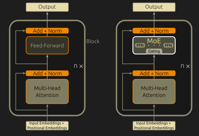
return results.view_as(inputs)The picture below shows the plain Transformer encoder architecture (left) and its MoE modified version (right). Block module is implemented by the Block class, which we will see shortly (actually there are n Block modules, n is coded as n_layer).
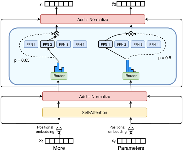
Below, a more detailed picture highlighting MoE layer (taken from https://arxiv.org/pdf/2101.03961.pdf). “Router” represents the gating module, experts are Feed Forward Networks (FFN 1, 2, 3 and 4).
Below, the code for the Transformer model (modified to include MoE layer). The Transformer consists of several blocks. So, to implement Transformer class, we need to implement the Block class first. In turn, to implement the Block class, we need MultiHeadAttention and FeedForward classes (other than MoeLayer, already defined). To define MultiHeadAttention we need the class Head.
class Head(nn.Module):
    def __init__(self, head_size):
        super().__init__()
        self.key = nn.Linear(n_embed, head_size, bias = False)
        self.query = nn.Linear(n_embed, head_size, bias = False)
        self.value = nn.Linear(n_embed, head_size, bias = False)
        self.register_buffer('tril', torch.tril(torch.ones(block_size, block_size)))
        self.dropout = nn.Dropout(dropout)

    def forward(self, x):
        B, T, C = x.shape
        k = self.key(x)
        q = self.query(x)
        wei = q @ k.transpose(-2, -1) * C**-0.5
        wei = wei.masked_fill(self.tril[:T, :T] == 0, float('-inf'))
        wei = F.softmax(wei, dim=-1)
        wei = self.dropout(wei)
        v = self.value(x)
        out = wei @ v
        return out

class MulitHeadAttention(nn.Module):
    def __init__(self, num_heads, head_size):
        super().__init__()
        self.heads = nn.ModuleList([Head(head_size) for _ in range(num_heads)])
        self.proj = nn.Linear(n_embed, n_embed)
        self.dropout = nn.Dropout(dropout)

    def forward(self, x):
        x =  torch.cat([head(x) for head in self.heads], dim=-1)
        out = self.dropout(self.proj(x))
        return out


class FeedForward(nn.Module):
    def __init__(self, n_embed):
        super().__init__()
        self.net = nn.Sequential(
            nn.Linear(n_embed, 4* n_embed),
            nn.ReLU(),
            nn.Linear(4 * n_embed, n_embed),
         nn.Dropout(dropout))

    def forward(self, x):
        return self.net(x)

class Block(nn.Module):
    def __init__(self, n_embed, n_head, num_experts=4):
        super().__init__()
        self.sa_head= MulitHeadAttention(n_head, n_embed//n_head)
        self.ffw = MoeLayer(
            experts=[FeedForward(n_embed) for _ in range(num_experts)],
            gate=nn.Linear(n_embed, num_experts, bias=False),
        )

        self.ln1 = nn.LayerNorm(n_embed)
        self.ln2 = nn.LayerNorm(n_embed)

    def forward(self, x):
        x = x + self.sa_head(self.ln1(x))
        x = x + self.ffw(self.ln2(x))
        return x


class Transformer(nn.Module):
    def __init__(self):
        super().__init__()

        self.token_embedding_table = nn.Embedding(vocab_size, n_embed, device=device)
        self.position_embedding_table = nn.Embedding(block_size, n_embed, device=device)
        self.blocks = nn.Sequential(*[Block(n_embd, n_head=n_head) for _ in range(n_layer)])
        self.lm_head = nn.Linear(n_embed, vocab_size)


    def forward(self, idx, targets=None):
        B, T = idx.shape

        token_emb = self.token_embedding_table(idx)
        pos_emb = self.position_embedding_table(torch.arange(T).to(device))
        x = token_emb + pos_emb
        x = self.blocks(x)
        logits = self.lm_head(x)
        if targets == None:
            loss = None
        else:
            B, T, C = logits.shape
            logits = logits.view(B*T, C)
            targets = targets.view(B*T)
            loss = F.cross_entropy(logits, targets)
        return logits, loss

    def generate(self, idx, max_new_tokes):
        for _ in range(max_new_tokes):
            idx_cond = idx[:, -block_size:]
            logits, loss = self(idx_cond)
            logits = logits[:, -1, :]
            probs = F.softmax(logits, dim = -1)
            idx_next = torch.multinomial(probs, num_samples = 1)
            idx = torch.cat((idx, idx_next), dim = 1)
        return idx
Here are all the necessary hyperparameters. max_iters is set to 3000 for testing (it will take some time to train). Probably things start to become significant for values larger than 5000…
# hyperparameters
batch_size = 64 # independent sequences processed in parallel
block_size = 256 # max context length
max_iters = 3000
eval_interval = 100
learning_rate = 1e-3
eval_iters = 200
n_embd = 384
n_embed = 384
n_head = 6
n_layer = 6
dropout = 0.0

# set device
device = 'cuda' if torch.cuda.is_available() else 'cpu'
Model training
Our model is the previously defined Transformer.
model = Transformer()The function below evaluates loss for training and validation data.
@torch.no_grad()
def estimate_loss():
    out = {}
    model.eval()
    for split in ['train', 'val']:
        losses = torch.zeros(eval_iters)
        for k in range(eval_iters):
            X, Y = get_batch(split)
            X = X.to(device)
            Y = Y.to(device)
            logits, loss = model(X, Y)
            losses[k] = loss.item()
        out[split] = losses.mean()
    model.train()
    return out
Move the model to the device and adopt AdamW optimizer.
model = model.to(device)
optimizer = torch.optim.AdamW(model.parameters(),lr=1e-4)
The training loop. If max_iters is large, it may take some time to complete.
for iter in range(max_iters):

    # print the loss on train and val datasets
    if iter % 100 == 0 or iter == max_iters - 1:
        losses = estimate_loss()
        print(f"step {iter}: train loss {losses['train']:.4f},
            val loss {losses['val']:.4f}")

    # sample a batch of data
    xb, yb = get_batch('train')
    xb = xb.to(device)
    yb = yb.to(device)

    # evaluate the loss
    logits, loss = model(xb, yb)
    optimizer.zero_grad(set_to_none=True)
    loss.backward()
    optimizer.step()
[OUTPUT]
step 0: train loss 4.9073, val loss 4.9073
step 100: train loss 2.3431, val loss 2.3454
step 200: train loss 2.3039, val loss 2.3042
step 300: train loss 2.2779, val loss 2.2779
step 400: train loss 2.2433, val loss 2.2438
step 500: train loss 2.1811, val loss 2.1828
step 600: train loss 2.0586, val loss 2.0600
step 700: train loss 1.8800, val loss 1.8853
step 800: train loss 1.7369, val loss 1.7424
step 900: train loss 1.6339, val loss 1.6397
step 1000: train loss 1.5603, val loss 1.5576
step 1100: train loss 1.4920, val loss 1.4932
step 1200: train loss 1.4438, val loss 1.4467
step 1300: train loss 1.3997, val loss 1.4049
step 1400: train loss 1.3656, val loss 1.3669
step 1500: train loss 1.3264, val loss 1.3289
step 1600: train loss 1.3024, val loss 1.2976
step 1700: train loss 1.2736, val loss 1.2743
step 1800: train loss 1.2499, val loss 1.2537
step 1900: train loss 1.2261, val loss 1.2253
step 2000: train loss 1.2046, val loss 1.2061
step 2100: train loss 1.1865, val loss 1.1890
step 2200: train loss 1.1698, val loss 1.1704
step 2300: train loss 1.1549, val loss 1.1545
step 2400: train loss 1.1383, val loss 1.1397
step 2500: train loss 1.1250, val loss 1.1214
step 2600: train loss 1.1100, val loss 1.1127
step 2700: train loss 1.0963, val loss 1.0971
step 2800: train loss 1.0880, val loss 1.0880
step 2900: train loss 1.0735, val loss 1.0768
step 2999: train loss 1.0622, val loss 1.0644Model evaluation
We test our model first encoding some small sequence d to get started.
d = 'a long time ago, there was a '
x = torch.tensor(encode(d), dtype = torch.long,device=device).unsqueeze(0)
print(decode(model.generate(x, max_new_tokes=500)[0].tolist()))
[OUTPUT]
a long time ago, there was a she what orn it was drawaying.
Lily said on the tress and went fast, what let so deep. So, he said, "From you, Max! I have full new get special?" But so atcher amaze her paint and hellped swing that mudre that he every day.
One Bunny day, a ball abloove make turn very thought animals alun. Lily asked the field mortor the ground, another of get theree were so aftul, scareful deond again.
One day, a mexe, something more sak yurng afr he could the make slove locks?
Lily asked her for to man stook Useful links
Code notebook (link)
Switch Transformers: Scaling to Trillion Parameter Models with Simple and Efficient Sparsity
W. Fedus, B. Zoph, N. Shazeer
arXiv:2101.03961v3 [cs.LG](2021, rev. 2022)
GShard: Scaling Giant Models with Conditional Computation and Automatic Sharding
D. Lepikhin, H. Lee, Y. Xu, D. Chen, O. Firat, Y. Huang, M. Krikun, N. Shazeer, Z. Chen
arXiv:2006.16668v1 [cs.CL] (2020)
TinyStories dataset (link)
Mixture of Experts Explained (link)