
PyTorch backward function
Small examples and more


This post examines some backward() function examples about the autograd (Automatic Differentiation) engine of PyTorch. As you already know, if you want to compute all the derivatives of a tensor, you can call backward() on it. The torch.tensor.backward function relies on the autograd function torch.autograd.backward that computes the sum of gradients (without returning it) of given tensors with respect to the graph leaves.
A first example
In a tutorial fashion, import torch library
import torchand consider the matrix
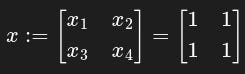
coded as
x = torch.ones(2, 2, requires_grad=True)and y defined as
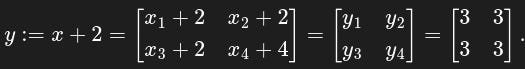
Note that, throughout the whole post, the asterisk symbol stands for entry-wise multiplication, not the usual matrix multiplication. Then we define z in terms of y:

Define out as the mean of the entries of z:
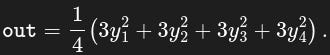
Important: out contains a single real value. This value is the result of a scalar function (in this case, the mean function).
y = x + 2
z = y * y * 3
out = z.mean()
Now, how do we compute the derivative of out with respect to x? First we type
out.backward() to calculate the gradient of current tensor and then, to return , we use
x.grad[OUTPUT]
tensor([[4.5000, 4.5000],
[4.5000, 4.5000]]) These values are obtained because, for example, taking the derivative w.r.t. one gets
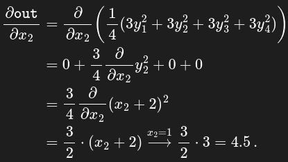
The zeros in the second row are due to the fact that and do not depend on , hence their derivative is zero. The grad attribute is None by default and becomes a tensor the first time a call to backward() computes gradients for self. The attribute will then contain the gradients computed and future calls to backward() will accumulate (add) gradients into it. Alternatively, use just
torch.autograd.grad(outputs=out, inputs=x)instead of x.grad, without calling backward(). What happens if you call, for example, z.grad or y.grad? Neither z nor y are graph leaves, so you will get no result and a warning (check next section).
A neural networks example
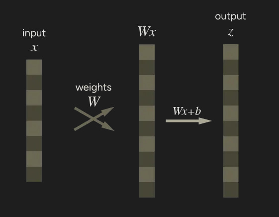
Neural networks use the backpropagation algorithm: neural network parameters (model weights) are adjusted according to the gradient of the loss function with respect to the given parameter. PyTorch has torch.autograd as built-in engine to compute those gradients. The engine supports automatic computation of gradients for any computational graph. Consider the simplest one-layer neural network, with input x, parameters W and b, and some loss function.
x = torch.ones(8)  # input tensor
y = torch.zeros(10)  # expected output
W = torch.randn(8, 10, requires_grad=True) # weights
b = torch.randn(10, requires_grad=True) # bias vector
z = torch.matmul(x, W) + b # output
loss = torch.nn.functional.binary_cross_entropy_with_logits(z, y)
We can represent the code with the following computational graph.
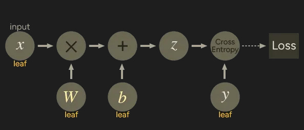
W and b are parameters, x is the input. We can only obtain the grad properties for the leaf nodes of the computational graph which have requires_grad property set to True. Calling grad on non-leaf nodes will elicit a warning message:
[OUTPUT]

UserWarning: The .grad attribute of a Tensor that is not a
leaf Tensor is being accessed. Its .grad attribute won't be
populated during autograd.backward().
Try it yourself typing:
loss.backward()
print(W.grad)
print(b.grad)
print(x.grad)
print(y.grad)
print(z.grad) # WARNING
print(loss.grad) # WARNING
Note that loss is a scalar output. Applying backward() directly on loss (with no arguments) is not a problem because loss represents a unique output and it is unambiguous to take its derivatives with respect to each variable in x. The situation changes when trying to call backward() on a non-scalar output. For example, consider the 10-entries tensor z. When calling backward() on it, what do you expect x.grad to be? We will address this problem in the following sections.
Vector-Jacobian product
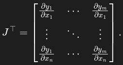
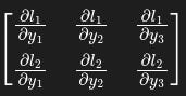
In general, torch.autograd is an engine for computing vector-Jacobian products, that is, the product J ᐪ ᐧ v where v is any vector and
If v happens to be be the gradient of a scalar function l=g(y), that is
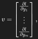
then the vector-Jacobian product returns the gradient of l with respect to x:
Let’s focus on our first example to understand what actually happens. Note that out from the first example is a scalar function just like the function l = g(y) previously cited: you can think of mean as g and out as l: out = mean(y₁, y₂, y₃, y₄). In our case, the Jacobian matrix is the following
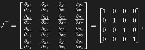
where yᵢ = xᵢ + 2 for i=1, 2, 3, 4. Since v is the vector of derivatives of out with respect to the yᵢ, the product Jᐪ ᐧ v is
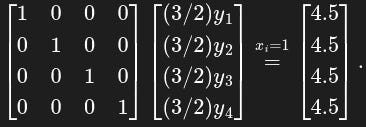
Therefore, the vector-Jacobian product returns x.grad , as expected.
The function torch.autograd.grad computes and returns the sum of gradients of outputs w.r.t. the inputs. If the output is not a scalar quantity, then one has to specify v, the “vector” in the Jacobian-vector product. Note that torch.autograd.grad is a method, torch.tensor.grad is a tensor attribute.
Example 1
Another example of vector-Jacobian product is the following. Here we suppose that v is the gradient of an unspecified scalar function l = g(y). The tensor v is defined by torch.rand(3).
import torch
x = torch.rand(3, requires_grad=True)
y = x + 2

# y.backward() <---
# RuntimeError: grad can be implicitly
# created only for scalar outputs
# try ---> y.backward(v) where v is any tensor of length 3

v = torch.rand(3)

y.backward(v)
print(x.grad)
Alternatively, just use
torch.autograd.grad(outputs=y, inputs=x, grad_outputs=v)instead of x.grad, without backward. Tensor v has to be specified in grad_outputs.
Example 2
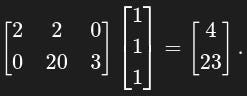
Let x = [x₁, x₂] and define y as
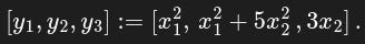
In this case the transposed Jacobian J ᐪ is
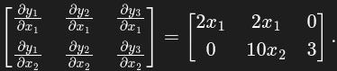
Now, assign numeric values to x₁ and x₂ setting x = [1, 2] and — since y is not a single scalar output — choose the vector v to be, for simplicity, [1, 1, 1]. The vector-Jacobian product is
This example is easily represented by the following code.
import torch
x = torch.tensor([1., 2], requires_grad=True)
print("x: ", x)

y = torch.empty(3)
y[0] = x[0]**2
y[1] = x[0]**2 + 5*x[1]**2
y[2] = 3*x[1]
print('y:', y)

v = torch.tensor([1., 1, 1,])
y.backward(v)
print('x.grad:', x.grad)
The general case
We have seen — and it is also shown on the official autograd page — that if you have a function and a vector happens to be the gradient of a scalar function , then the vector-Jacobian product would be the gradient of with respect to . But what happens when is not a simple vector? Consider the following code.
x = torch.tensor([[1.,2,3],[4,5,6]], requires_grad=True)
y = torch.log(x)
# y is a 2x2 tensor obtained by taking logarithm entry-wise

v = torch.tensor([[3.,2,0],[4,0,1]], requires_grad=True)
# v is not a 1D tensor!

y.backward(v)
x.grad # returns dl/dx, as evaluated by "matrix-Jacobian" product v * dy/dx

# therefore we can interpret v as a matrix dl/dy
# for which the chain rule expression dl/dx = dl/dy * dy/dx holds.
[OUTPUT]
tensor([[3.0000, 1.0000, 0.0000],
[1.0000, 0.0000, 0.1667]]))Here is a function of the 2×3 matrix . The function is obtained applying entry-wise the natural logarithm to the elements of . As you can see, in this case is not a simple vector, it’s a 2×3 matrix. So how to interpret ? Here can be interpreted as the tensor
such that when performing entry-wise matrix-Jacobian one gets
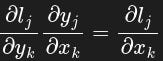
in a chain-rule fashion. Hence, when calling x.grad, we obtain the result of the entry-wise product of by :
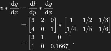
For the “Jacobian” — it is not the actual Jacobian, that would be a 6×6 matrix including all the ∂yᵢ/∂xⱼ, it is a matrix composed of the Jacobian diagonal entries— remember that the derivative of log(z) is 1/z. Note that x.grad is equivalent to the (entry-wise) product v*(1/v) where the matrix 1/v contains the reciprocals of entries in v.
The math in PyTorch autograd’s tutorial page about vector-Jacobian product is fine but may be misleading in cases like the latter example: what PyTorch actually evaluates is an entry-wise product between (interpreted as the matrix containing derivatives of function with respect to ) and the matrix (the matrix containing the derivatives of with respect to ).
Useful links
torch.autograd - PyTorch Docs (link)
torch.autograd.backward - PyTorch Docs (link)