


The Kullback-Leibler divergence
A fundamental comparison tool


In this post we will just spend a few words on a well-known measure of how dissimilar a given distribution is from another reference distribution. First we will give a definition for such a measure and then we will provide some intuitive meaning together with some useful coding snippets.
Definition
Let’s begin with the discrete case. So let P and Q be two probability distributions defined on the same probability space . A first attempt may be considering the average of the difference between the distributions. Quite close indeed, the following defintion is just a little bit different. The Kullback-Leibler divergence (also called relative entropy) KL(P ‖ Q) is defined as the average of the difference between the logarithms of probabilities P(x) and Q(x):
The expectation is taken using the probabilities P (often written as x ~ P). The definition of expectation leads to the expression
In the case of continuous distributions we write
where p(x) and q(x) are P and Q respective densities.
KL divergence is often called a “distance” but it is not a distance in mathematical sense (a metric): KL divergence is not symmetrical. This means that KL(P ‖ Q) is generally different from KL(Q ‖ P).
If Q(x) is 0 for some x, the KL divergence is not defined unless P(x) = 0. What if P is 0 somewhere? In this case, we interpret that the KL divergence must be zero since when a approaches 0, the expression alog(a) tends to 0 .
Motivations behind the definition
A first intuition comes form the fact that if {pi} and {qi} are two probability mass functions, that is, two countable or finite sequences of nonnegative numbers that sum to one, then
with equality if and only if pi = qi for all i. The fact that the divergence of a probability distribution with respect to another one is nonnegative and zero only when the two distributions are the same suggests the interpretation of KL divergence as a “distance” between two distributions, that is, a measure of how different the two distributions are.
A second intuition about the fact that KL divergence actually expresses some kind of distance between two distributions comes from the expression
where it is immediate to recognize that the difference between logarithms D(x) is a term expressing the gap between the two distributions. If the average gap is small, then the two distributions are “similar” or “close”.
Connection with cross entropy
KL divergence KL(P ‖ Q) is equal to
where H(P , Q) is the cross entropy of P and Q and H(P) is the entropy of P. As we said, KL(P ‖ Q) can be thought of as something like a measurement of how far the Q distribution is from the P distribution. But cross entropy is itself such a measurement… the difference is that cross entropy has a — generally nonzero — minimum when P = Q, that is H(P , P) = H(P); so in KL divergence we subtract the entropy term H(P) to attain minimum value 0. This is coherent with the property that the distance of an object from itself should be zero.
Quick example
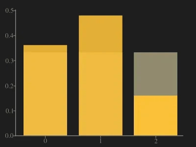
Let P and Q be the following distributions (each possible outcome x is in = {0, 1, 2}):
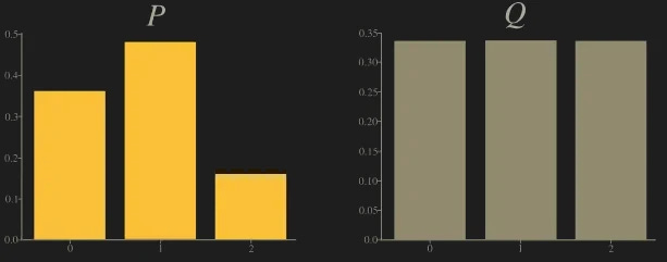
The following picture shows both P (amber) and Q (gray).
Next picture shows the logarithm of distributions with the difference D at x = 2.
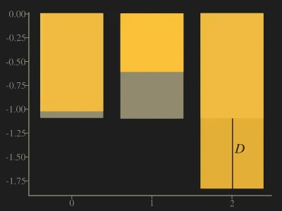
Let’s calculate KL(P ‖ Q).
Interchanging the arguments, we find that KL(Q ‖ P) is approximately 0.0974 and this value is different from the previous.
Evaluate KL divergence with Python
Import the entropy function
from scipy.stats import entropyand then compute KL(P ‖ Q) from the example above in just one line.
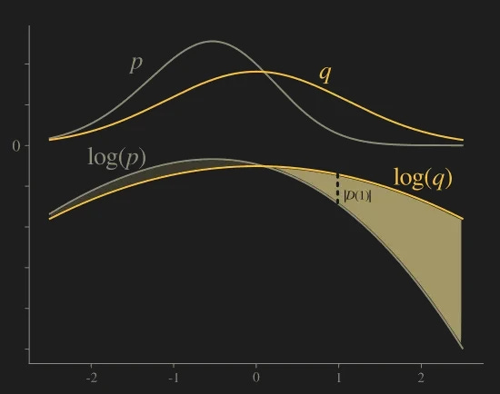
entropy([9/25, 12/25, 4/25], qk=[1/3, 1/3, 1/3])0.0852996013183706Below, a simple Python coding example for figures 1~4. Note that the two continuous density curves have a magnifying coefficient for scaling purposes.
import matplotlib.pyplot as plt
import numpy as np

p = [9/25, 12/25, 4/25]
q = [1./3,1./3,1./3]
xx = ['0','1','2']

logq = np.log(q)
logp = np.log(p)

plt.bar(xx, q, color='beige')
plt.bar(xx, p, alpha=.6, color='yellowgreen')
plt.show()

plt.bar(xx, logq, color='beige')
plt.bar(xx, logp, alpha=.6, color='yellowgreen')
plt.show()
from scipy.stats import norm, skewnorm
x = np.arange(-3,2.5,.001)
plt.plot(x, 10*skewnorm.pdf(x,-1.2), color='black')
plt.plot(x, 10*norm.pdf(x, scale=1.1), color='yellowgreen')
log1 = np.log(skewnorm.pdf(x,-1.2))
log2 = np.log(norm.pdf(x, scale=1.1))
plt.plot(x, log1, color='black')
plt.plot(x, log2, color='yellowgreen')
plt.fill_between(x, log1, log2,
where=log1>=log2, facecolor='darkgrey',
interpolate=True)
plt.fill_between(x, log1, log2,
where=log1<log2, facecolor='lightgreen',
interpolate=True)
plt.show()
Mean-seeking and mode-seeking
As we have noted, the KL-divergence is not symmetric. There are some substantial differences between the forward Kullback-Leibler divergence KL(P || Q) and the reverse Kullback-Leibler divergence KL(Q || P), at least as far as their minimization is concerned.
The forward KL divergence is minimized when Q is more spread out, covering all P. So the forward KL is described as mean-seeking. To understand the reason, we look at the expression forward KL divergence. For a target distribution q(x), taking into account the expression of forward KL, if there is an x where q(x) is significantly greater than zero and p(x) is very close to zero, then q(x) log(q(x)/p(x) ) is large. Therefore, to keep the forward KL small, whenever q is large, then we also need a large p.
On the other hand, the reverse KL integrates the expression p(x) log( p(x)/q(x) ), and even if q(x) is significantly greater than zero, we can choose p(x) = 0 without p(x) log(p(x)/q(x) ) becoming large. This means that if Q is multi-modal, P can select one mode. This may be desirable in RL, because it can concentrate the action probability on the region with the highest value, even if there is another region with rather high action values. That’s why reverse KL is described as mode-seeking.
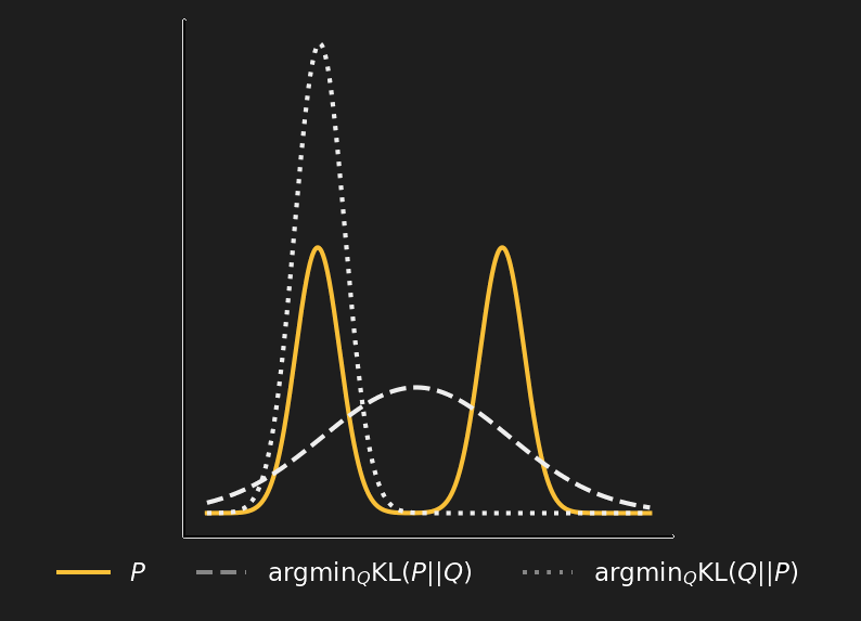
The figure above is a clear picture of how things stand with the two KL divergences. P is a multimodal distribution, KL(P || Q) is minimized if Q is spread out (dashed line); KL(Q || P) is minimized if Q is concentrated in one mode.